|
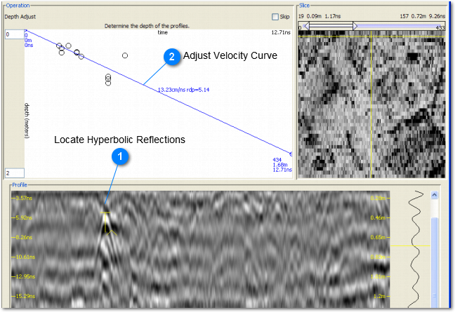
The timescal (ns) in GPR data can be converted to depth using an average velocity. Velocity can be estimated based on the dimensions of a hyperbolic reflections. This step requires at least one hyperbolic reflection, and preferable several.
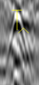
 Locate Hyperbolic Reflections
Scroll through each profile to find hyperbolic reflections such as this one. Each one can be used to calculate a velocity for that location. Click (left-click) at the apex of the hyperbola. You will see a "T" symbol appear. Next, right click at some point along the tail of the hyperbola. A "^" symbol will appear. Each time this is done a circle appears in the chart above. If you click on the tail of the same hyperbola multiple times, new velocity calculations will be made each time. Find several hyperbolas in different profiles and depths in your dataset and go through this process. When done, you should have a graph in the Operation window showing all the velocity points. There may be some outliers but hopefully there is a trend.
|
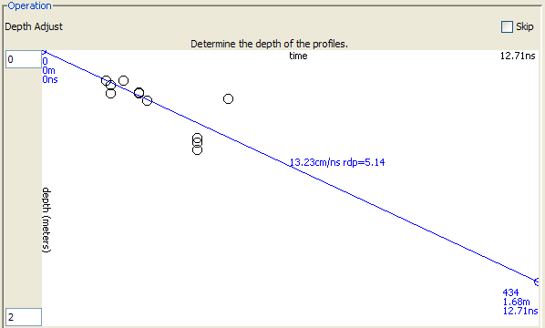
 Adjust Velocity Curve
The blue line can be adjusted to best fit the points on the graph. To so so, drag the right-most blue circle (handle) and move up and down until you have a line of best fit. (It was found that this is better than computing a best fit lie becuase you can ignore outliers and choose points along the curve to mark velocity chages. To make the line fit you can try two other tactics. First, change the depth maximum in the lower-left corner. Increase the number to make more room for dragging the bottom of the velocity line downwards, or decrease the number to show more detail in your graph. Finally, you can add more dots (handles) along the velocity curve, if it appears that velocity changes with depth (which it usually does, but it is hard to find hyperbolic reflections at a variety of depths to show this).
|
|
|